Predicting Virus Relative Abundance in Wastewater
Jeff Kaufman, Dan Rice, Simon Grimm, and Mike McLaren
August 10th, 2023
Thanks to Asher Parker-Sartori for assistance in collecting public health estimates, to Will Bradshaw and Charlie Whittaker for helpful feedback on this report, and to the authors[1] of the metagenomics papers we analyzed for collecting this data and making it publicly available.
Summary
At the Nucleic Acid Observatory (NAO) we're evaluating pathogen-agnostic surveillance. A key question is whether metagenomic sequencing of wastewater can be a cost-effective method to detect and mitigate future pandemics. In this report we investigate one piece of this question: at a given stage of a viral pandemic, what fraction of wastewater metagenomic sequencing reads would that virus represent?
To make this concrete, we define . If 1% of people are infected with some virus (prevalence) or have become infected with it during a given week (incidence), is the fraction of sequencing reads (relative abundance) generated by a given method that would match that virus. To estimate we collected public health data on sixteen human-infecting viruses, re-analyzed sequencing data from four municipal wastewater metagenomic studies, and linked them with a hierarchical Bayesian model.
Three of the viruses were not present in the sequencing data, and we could only generate an upper bound on . Four viruses had a handful of reads, for which we were able to generate rough estimates. For the remaining nine viruses we were able to narrow down for a specific virus-method combination to approximately an order of magnitude. We found for these nine viruses varied dramatically, over approximately six orders of magnitude. It also varied by study, with some viruses seeing an three orders of magnitude higher in one study than another.
The NAO plans to use the estimates from this study as inputs into a modeling framework to assess the cost effectiveness of wastewater MGS detection under different pandemic scenarios, and we include an outline of such a framework with some rough estimates of the costs of different monitoring approaches.
Introduction
With the COVID-19 pandemic there's been a large increase in wastewater monitoring for tracking the prevalence of different infectious diseases. Most of this work has focused on tracking known pathogens, but at the NAO we're interested in whether we can detect novel ones, even potentially ones intentionally engineered to evade screening. This means that standard strategies like quantitative PCR, which allow you to measure the concentration of nucleic acids containing a known pattern of bases, aren't a good fit for our goals. Instead, we've been exploring metagenomic sequencing because it's relatively pathogen-agnostic. We could sequence many samples, identify suspicious sequences computationally, and flag them for further analysis. For more details, see our 2021 preprint, A Global Nucleic Acid Observatory for Biodefense and Planetary Health.
If this were run at a large scale, we expect the largest cost to be sequencing. Thus, narrowing down how much sequencing this approach might require would help figure out whether and how this effort is worth pursuing. Since detection requires sequencing reads that match the target virus, the largest determinant of sequencing quantity is relative abundance: the fraction of sequencing reads that match a target. Going into this project we had a rough estimate, from SARS-CoV-2 in a single paper, for what sort of relative abundance you might see at a given stage of an outbreak, and our goal with this project was to get a clearer picture of how epidemiological conditions translate into relative abundance.
Overall Approach
We approached this problem by combining existing metagenomic and public health data. We proceeded in five stages, each of which we describe more below:
Collect existing wastewater metagenomic sequencing data.
Identify target viruses.
Process the sequencing data to determine the relative abundance of each target virus.
Collect prevalence and incidence estimates from public health sources for these viruses.
Make statistical estimates for how these estimates translate into relative abundance.
Metagenomic Data Identification
We reviewed the literature for studies that: (a) performed shotgun metagenomic sequencing of municipal wastewater influent, (b) produced a large number of sequencing reads, and (c) published their data to the SRA. Our search wasn't exhaustive: our goal was to collect enough data to work with, not to survey everything.
We identified sixteen candidate papers (Table 1). In cases where they sampled from municipal treatment plants we discarded non-influent samples (ex: treated sludge, effluent). After running the data from these papers through our bioinformatics pipeline (see Appendix B) we saw that these papers varied enormously in the fraction of reads that we could assign to human viruses:
Table 1: Studies considered for this report, by country, relevant read count, and relative abundance of human viruses for eligible samples
| Paper | Sequencing | Country | Eligible Read Pairs | Relative Abundance of Human Viruses |
|---|---|---|---|---|
| Yang et al. (2020) | RNA | China | 1e+9 | 2e-4 |
| Cui et al. (2023) | Combined | China | 4e+7 | 8e-6 |
| Hendriksen et. al. (2019) | Combined | Kenya | 2e+9 | 8e-6 |
| Munk et al. (2022) | DNA | Multiple | 4e+10 | 6e-6 |
| Rothman et al. (2021) | RNA | United States | 7e+8 | 4e-6 |
| Crits-Christoph et al. (2021) | RNA | United States | 3e+8 | 3e-6 |
| Spurbeck et al. (2023) | RNA | United States | 2e+9 | 3e-6 |
| Brumfield et al. (2022) | DNA, RNA | United States | 5e+8 | 2e-6 |
| Brinch et al. (2020) | DNA | Denmark | 4e+9 | 2e-6 |
| McCall et al. (2023) | Combined | United States | 7e+7 | 2e-6 |
| Maritz et. al. (2019) | DNA | United States | 2e+8 | 1e-6 |
| Ng et al. (2019) | DNA | Singapore | 3e+8 | 3e-7 |
| Wang et al. (2022) | DNA | Saudi Arabia | 8e+9 | 2e-7 |
| Fierer et al. (2022) | DNA | United States | 1e+9 | 2e-7 |
| Petersen et al. (2015) | DNA | Multiple | 2e+9 | 1e-7 |
| Bengtsson-Palme et al. (2016) | DNA | Sweden | 7e+8 | 9e-8 |
Three studies, Crits-Christoph et al. (2021), McCall et al. (2023), Rothman et al. (2021), also included some samples where they performed amplification with a panel of primers intended to match specific genetic sequences:
Table 2: Effect of panel-amplification on relative abundance of human viruses. The second and third columns show the relative abundance of human viruses in all reads from panel-amplified samples and from (non-panel-amplified) eligible samples. All three studies performed RNA sequencing.
| Paper | Panel-amplified samples | Eligible samples | Amplification Ratio |
|---|---|---|---|
| Crits-Christoph et al. (2021) | 1e-2 | 3e-6 | 4000x |
| McCall et al. (2023) | 1e-3 | 2e-6 | 600x |
| Rothman et al. (2021) | 4e-5 | 4e-6 | 8x |
Panel amplification (Table 2) can give much higher relative abundance of human viruses. However, as we are interested in the performance of methods detecting novel viruses, which are unlikely to match these amplification primers, it is not a method we considered further and we excluded panel-amplified samples from the rest of our analysis.
Filtering Studies by Size, Public Health Data, and Sample Preparation
We then filtered these candidate studies to choose a set for deeper analysis. We were interested in ones with (a) many sequencing reads, (b) where we would be able to link samples to reliable public health estimates, and (c) where the sample preparation and sequencing are suitable for detecting a novel viral pathogen. Since most nucleic acids in wastewater are bacterial, and viruses in general have a very low relative abundance, we were especially interested in library preparation that could increase the viral fraction without resorting to overly specific methods like panel amplification. An example is the use of a 0.22 μm filter to remove bacteria and solids in Rothman et al. (2021). Three studies did well on these criteria: Crits-Cristoph et al. (2021), Rothman et al. (2021), and Spurbeck et al. (2023) (henceforth “Crits-Cristoph”, “Rothman”, and “Spurbeck”).
These three studies all performed only RNA sequencing: none of the candidate DNA sequencing studies included a step that seemed likely to bias sequencing towards viruses relative to bacteria. While even DNA-based viruses generate RNA and we did end up seeing DNA-based human viruses in the RNA sequencing data, we also wanted to evaluate DNA sequencing. Thus we decided to additionally include Brinch et al. (2020) (henceforth “Brinch”), as this represented the largest DNA sequencing dataset we could find from a location where we could get good public health data (Copenhagen, Denmark).
Table 3: Chosen studies, with metadata on the subset of samples we analyze in this report.
| Paper | Sequencing | # Reads included in report | # Samples included in report | Location | Dates |
|---|---|---|---|---|---|
| Brinch et al. (2020) | DNA | 4.4B pairs | 322 | Copenhagen, Denmark | 2015-11-20 to 2018-11-27 |
| Rothman et al. (2021) | RNA | 660M pairs | 97 | Los Angeles, CA, USA | 2020-07-20 to 2021-01-04 |
| Spurbeck et al. (2023) | RNA | 1.8B pairs | 55 | Ohio, USA | 2021-12-05 to 2022-01-09 |
| Crits-Christoph et al. (2021) | RNA | 298M pairs | 7 | San Francisco, CA, USA | 2020-06-30 to 2020-07-01 |
Terminology note: when we say "read", here and below, we mean a paired-end forward and reverse read pair. Each read pair corresponds to, modulo duplication during library prep and sequencing, an independent observation from the sample.
The three RNA studies all used 24-hour composite samples, while Brinch used 12-hour composites. Brinch, Spurbeck[2], and Rothman sampled from wastewater treatment plants (WTPs), while Crits-Cristoph sampled from interceptor lines. All four sequenced with paired-end Illumina technology. [3]
Target Viruses
We initially looked for viruses where we could get reasonable public health estimates for incidence or prevalence, and where we expected they would be common enough in the population that there was a chance of seeing them in the sequencing data. This first round gave us, categorized by mode of transmission:
Respiratory:
SARS-CoV-2: a coronavirus that causes COVID-19.
Influenza, types A and B: orthomyxoviruses, the most common causes of the flu.
Bodily fluids:
Human Immunodeficiency Virus (HIV): a retrovirus that causes AIDS.
Hepatitis B Virus (HBV): a hepadnavirus that causes the liver disease Hepatitis B.
Hepatitis C Virus (HCV): a flavivirus that causes the liver disease Hepatitis C.
Herpes Simplex Virus 1 (HSV-1): a herpes virus that causes cold sores.
Herpes Simplex Virus 2 (HSV-2): a herpes virus that causes genital herpes.
Epstein-Barr virus (EBV): a herpes virus that causes infectious mononucleosis
Cytomegalovirus (CMV): a herpes virus that causes a range of symptoms.
Fecal-oral:
Norovirus, genogroups I and II: caliciviruses that cause gastroenteritis.
Skin:
Human Papilloma Virus (HPV): a family of papillomaviruses that cause warts.
In selecting these viruses we considered what public health data was available, including whether it was available for times and places corresponding to the metagenomic sequencing data we collected. We did not consider whether the sequencing data contained any reads for these viruses because we didn't want to bias our estimates.
Later, after several of these viruses did not match any sequencing reads in the three virally-enriched datasets, we selected a second round of viruses, expanding our target set by six. Four of these we added because of their high number of reads in those three datasets:
Adeno-associated virus 2 (AAV2): a common parvovirus with likely benign effects.
BK virus (BKV), JC virus (JCV), and Merkel cell polyomavirus (MCV): common polyomaviruses that are likely benign unless the host is immunocompromised.
The other two, adeno-associated viruses 5 and 6 (AAV5, AAV6), we added because we came across good estimates for them in collecting an estimate for AAV2. Note that AAV5 was not present in the metagenomic sequencing data.
We later dropped HSV-2, HBV, and AAV6 from our analysis because our bioinformatics system wasn't capable of assigning reads to these viruses; see Appendix B: Bioinformatic Details.
In interpreting our results, be aware of the selection bias in these second-round viruses, especially AAV2, BKV, and JCV which were added for their high abundance. Similarly prevalent viruses that shed less into stool or were less amenable to the sequencing approaches used would not have been selected for study.
Bioinformatics
For the four studies we chose, we downloaded the raw reads from SRA, cleaned them with AdapterRemoval2, and classified them with Kraken2. We validated our assignments by verifying that (a) our Kraken2 configuration could classify simulated reads from each target virus and (b) reads assigned to each virus aligned well with the virus's genome. See Appendix B for more details.
Table 4: target viruses, showing nucleic acid type, selection round, the fraction of samples in each study with at least one matching read and, in parentheses, the total number of matches across all samples.
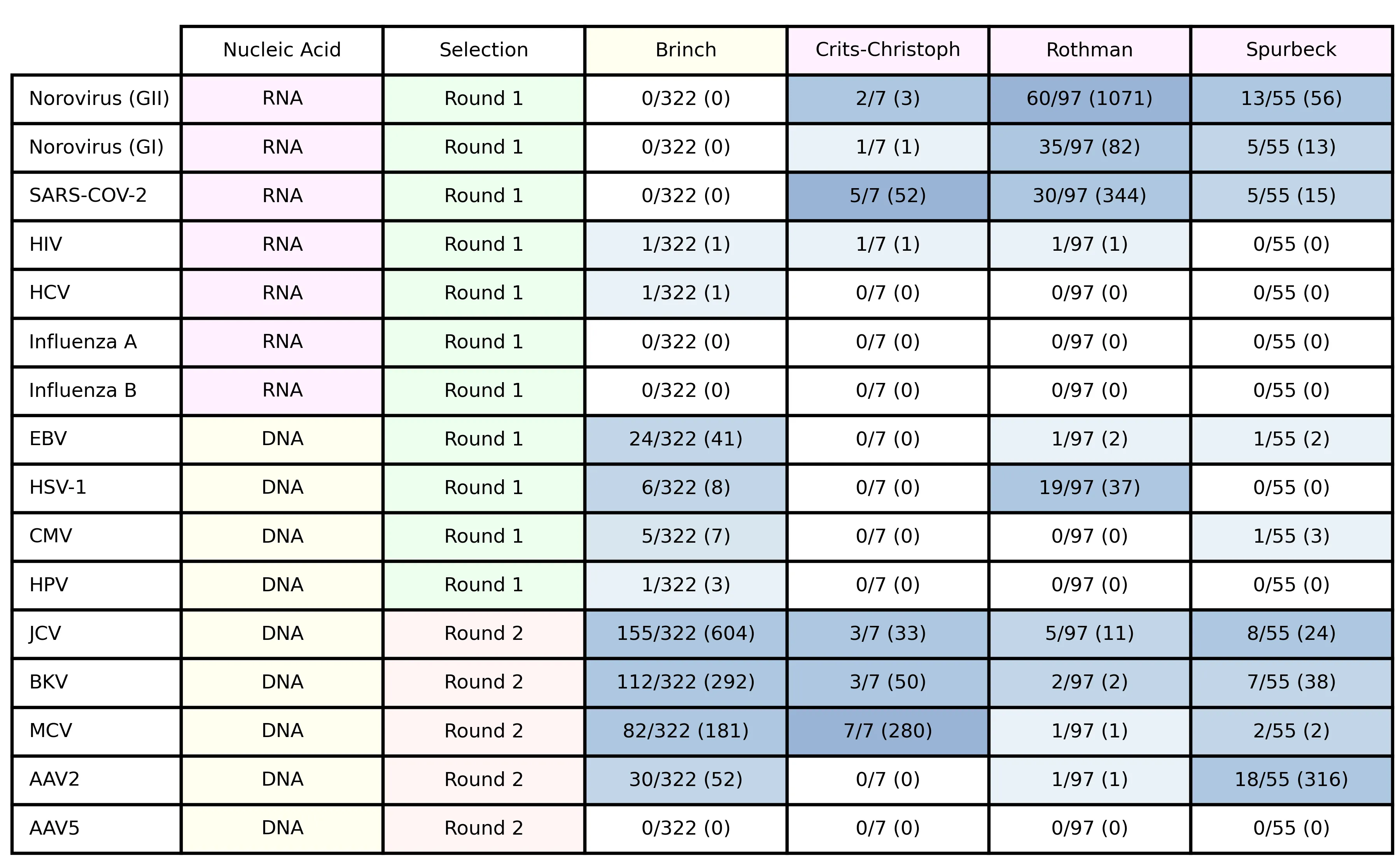
Several viruses had few or no matches. In general, results drawing on these counts will be most robust for viruses with many matches.
Public Health Data
Depending on the data available for a virus, we collected public health data to estimate one of two related quantities:
Prevalence: the fraction of people infected at the time of sample collection
Weekly incidence: the fraction of people acquiring the infection in the week leading up to sample collection
We found public health sources gave prevalence data for infections that are typically chronic and incidence otherwise, so we estimated prevalence for chronic-infection viruses and incidence for acute-infection ones.[4] For all estimates, we used a custom machine-readable system to make public health data and subsequent calculations easily reviewable and reproducible.
Prevalence estimates
When estimating virus prevalence, we sought high-quality data matching the time and country[5] of each metagenomic sample as closely as possible. First, we looked for prevalence estimates from public health agencies for the target pathogen, time, and location. If one wasn't available we next tried to generate one by reanalyzing the data from cohort studies, e.g., seroprevalence measurements. When there were no estimates or data for the target time, we looked for data for the same location at another time. Finally, if data for the target location couldn’t be found for any time, we expanded our search to different locations with similar demographics.
A full run-down of data sources and methods for each estimate can be found in Appendix A; specific data sources and calculations are detailed on GitHub.
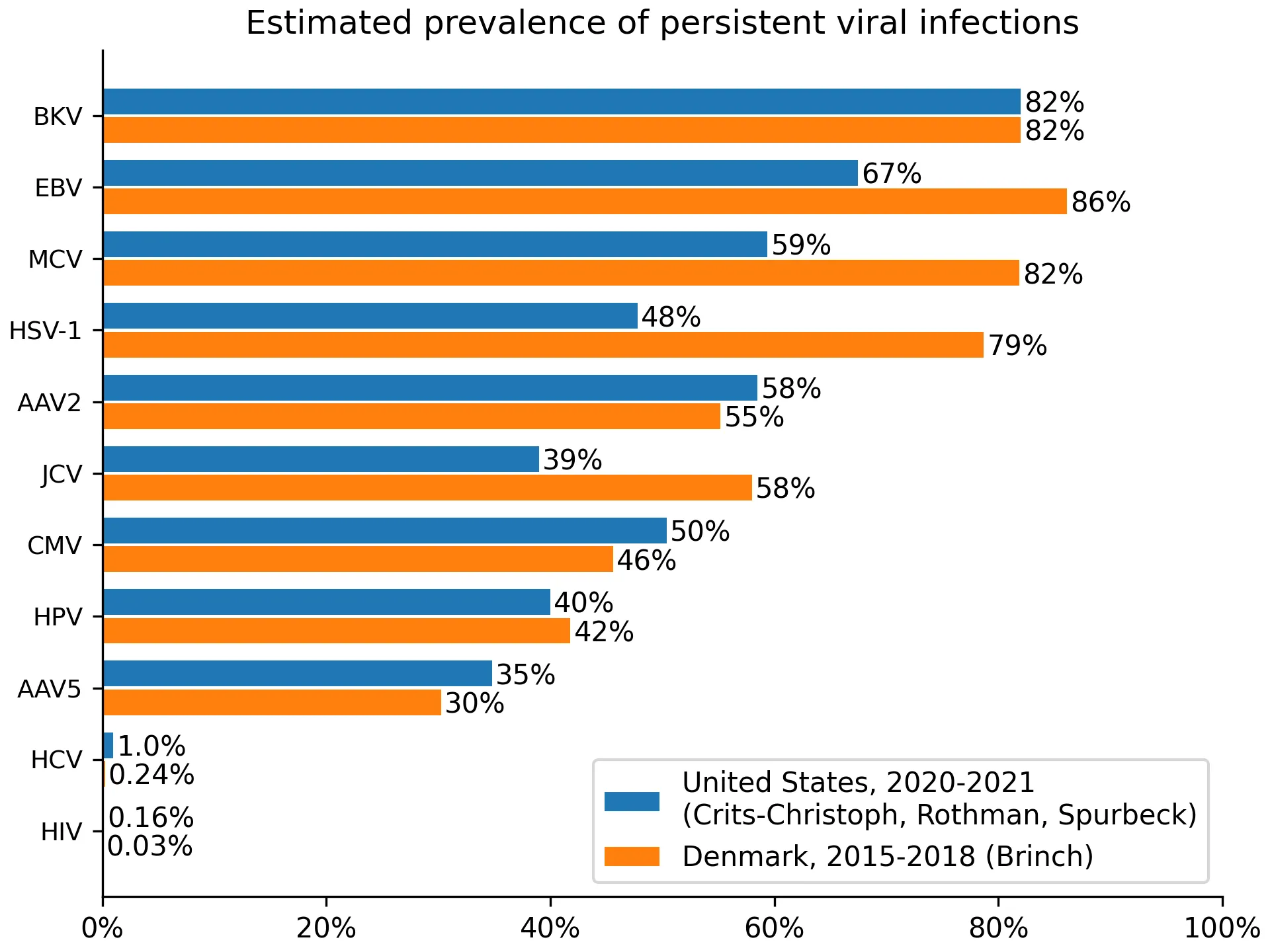
As an overview, for US estimates we found good prevalence estimates for Human Immunodeficiency Virus (HIV), Hepatitis B Virus (HBV), Hepatitis C Virus (HCV), and Herpes Simplex Virus 1 and 2. We used seroprevalence data—the share of individuals with antibodies against the virus—for Cytomegalovirus (CMV), and Epstein-Barr-Virus (EBV). We used PCR testing data for Human Papilloma Virus (HPV). This seroprevalence and PCR data was collected in the National Health and Nutrition Examination Survey (NHANES), a biannual health survey of a US population sample that includes testing for common chronic infections.
For viruses of lower public-health concern, estimates were not generally available from these sources. We expanded our search to individual seroprevalence studies (AAV-2, AAV-5, AAV-6, John-Cunningham Virus (JCV), BK Virus (BKV) and Merkel Cell Virus (MCV)).
For Denmark, we often didn’t identify prevalence estimates, so we instead used seroprevalence measurements. Seroprevalence measurements overestimate prevalence because some people clear the virus but retain antibodies. This is visible when comparing EBV or HSV-1 estimates between the US and Denmark, with Denmark showing higher prevalence. Ideally, we would have adjusted for this effect, but we did not find estimates of its size. When we didn’t identify either prevalence estimates or seroprevalence measurements from Denmark, we identified the best data source from a country with similar demographic, e.g., Switzerland (BKV), the Netherlands (MCV), or Germany (HSV-1). The resulting prevalences can be found in Figure 1.
Figure 1: estimated prevalence for viruses where we collected prevalence data.
Incidence estimates
For acute, seasonal virus infections (influenza, SARS-CoV-2, norovirus) we estimated incidence rates. We only created these estimates for the US. We did not generate estimates for Denmark primarily because we did not expect to see (and, in fact, did not see) any matching reads in Brinch: their sampling predates the emergence of SARS-CoV-2, and norovirus and influenza are non-reverse-transcribing RNA-based viruses. Additionally, collecting a set of public health estimates for a seasonal pathogen in a new country involves substantial effort to understand surveillance and data sharing standards.
Compared to estimating the prevalence of chronic viruses, estimating the incidence of acute ones is harder because there's much more variance over space and time. We first tried to identify incidence estimate time-series data, if possible on a state or county-level. This data was unavailable, and we thus looked for alternative indicators of disease activity. In the case of SARS-CoV-2 and influenza these were the number of daily (SARS-CoV-2) and weekly (influenza) confirmed positive tests, for norovirus it was the number of outbreaks per month.
Testing efforts and outbreak reporting frequently miss infections. To adjust for such underreporting we took two approaches. For SARS-CoV-2 we used an official uniform underreporting factor provided by the CDC, multiplying the 7-day moving average of daily confirmed cases with this figure[6]. In the case of influenza and norovirus, we began by aggregating all reported positive tests or outbreaks across a given year. For each week or month, we then calculated the fraction of outbreaks or positive tests occurring in that timeframe, multiplying this fraction with the estimated annual number of influenza or norovirus cases, as reported by the CDC.
Through this process, we arrived at daily SARS-CoV-2 incidence rates with county-level resolution, influenza incidence rates with state-wide weekly[7] resolution, and norovirus incidence rates with national monthly resolution, plotted in Figure 2.
Figures 2a and 2b: Estimated incidence for acute infecting viruses and study coverage
_Z11I3ee.webp)
_Z2p1l9r.webp)
As seen in Figure 2b, influenza was suppressed from March 2020 to November 2022. This decrease was most likely driven by COVID-19 public health measures.[8]
Statistical Analysis
Overview of Approach
Our objective was to determine how the relative abundance of a virus in a wastewater metagenomic sample varies as a function of either prevalence or incidence (collectively, the public health predictor). First, we wrote a simple deterministic model that relates the expected relative abundance to the public health predictor. Second, we used this deterministic model to develop a hierarchical Bayesian model that accounts for key sources of random variation in the public health predictor and metagenomic measurements. Third, we implemented the Bayesian model in the Stan statistical programming language, and fit it separately for each virus and study. Finally, we used the fitted model to estimate summary statistics, including : the relative abundance of a target virus when the public health predictor is at 1% of the population.
Predicting Expected Relative Abundance
As the basis for statistical inference we began by defining a simple deterministic model predicting relative abundance as a function of the public health predictor. Relative abundance is the fraction of all reads that were assigned to the focal virus:
The expected relative abundance of a virus in a metagenomic sample depends on a variety of factors, including
The (true) public health predictor: the fraction of people in the relevant population (e.g., the catchment of the WTP) who are currently and/or have recently been infected with the virus.
How much of the virus that an infected person sheds, relative to the background microbiome that everyone sheds.
Nucleic acids in wastewater from sources other than human shedding, such as runoff or rodents.
Intrinsic bias in the metagenomic protocol that may favor or disfavor the virus relative to the background microbiome.
We assume the relationship
where is a constant of proportionality that accounts for factors 1 through 4, along with other factors that might affect the apparent abundance of the virus relative to everything else in the sequencing data at a given level for the public health predictor. Intuitively, the constant describes the approximate increase in relative abundance per unit increase in the public health indicator (with the approximation being valid when the relative abundance much less than 100%). In our results below, we instead consider the the expected relative abundance of the virus when the public health predictor equals one person per hundred, which we denote as . The above equation implies that , and scales approximately linearly (e.g. ) so long as .
Bayesian Model and Estimation
We estimated (and ) separately for each virus and study, taking the read counts and our estimates of the public health indicator as inputs. We used a hierarchical Bayesian logistic regression model, described in detail in Appendix C: Statistical Analysis Details. This model was designed to be the simplest model that:
Captures the discrete count nature of sequencing data by modeling the counts with a binomial distribution,
Allows for additional random variation in the read counts (beyond that implied by the binomial distribution), due to sample collection and processing,
Allows for random error in our estimate of the public health indicator for that sample, and
Allows for variation in the constant by location within a study.
The hierarchical model allows us to jointly estimate the location-specific effects and an overall coefficient for the study and virus. We fit the model using the PyStan interface to the Stan statistical programming language. Stan uses a Hamiltonian Monte Carlo algorithm to generate samples from the joint posterior distribution of the model parameters.
Because the model worked in log space, it was unable to handle cases where a public health predictor was zero. Due to a combination of the COVID-19 pandemic and some samples being taken outside of typical flu season, our public health sources gave us weekly counts of zero for influenza A for 100% of Crits-Christoph samples, 35% of Rothman samples, and 23% of Spurbeck samples. Influenza B was even less common, with weekly counts of zero for 100% of Crits-Christoph samples, 55% of Rothman samples, and 36% of Spurbeck samples. We handled these weeks with a "pseudocount", by telling the model to assume that in weeks when there were 0 reported cases there were actually 0.1 cases.
Modeling Results
Our main summary statistic is , the expected relative abundance at 1:100 prevalence or weekly incidence. We denote these as and , respectively. In figures 3 and 4 we've plotted the posterior distributions of and for all viruses across the four MGS studies. We've plotted posterior estimates that are based on fewer than ten reads from the focal virus in a paler color, to indicate that readers should take them less seriously.
A text file with summary statistics of the posterior distributions is available in our GitHub repository.
For viruses with no observed reads (e.g., influenza A and B), the left tail of the distribution does not contain substantive information. In these cases, we mark it with vertical hatching to indicate that we do not have a meaningful estimate of the lower bound on . The right tails of these distributions, however, do contain useful information: given the total number of reads in a study, failing to observe a virus puts an upper bound on .
In the two cases where we used pseudocounts (influenza A and B) the right tail could be driven by the choice of pseudocount: a smaller value would give a higher upper bound on . We performed a sensitivity analysis[9], and determined that this only had a substantial impact on our estimate for Crits-Christoph. We dropped our Crits-Christoph influenza estimates from our analysis below.
Expected Relative Abundance by Virus and Study
Here are the posterior distributions of for viruses with incidence estimates. These are the seasonal RNA-based viruses, which we identified in our first selection round:
Figure 3: for viruses where we estimated incidence.
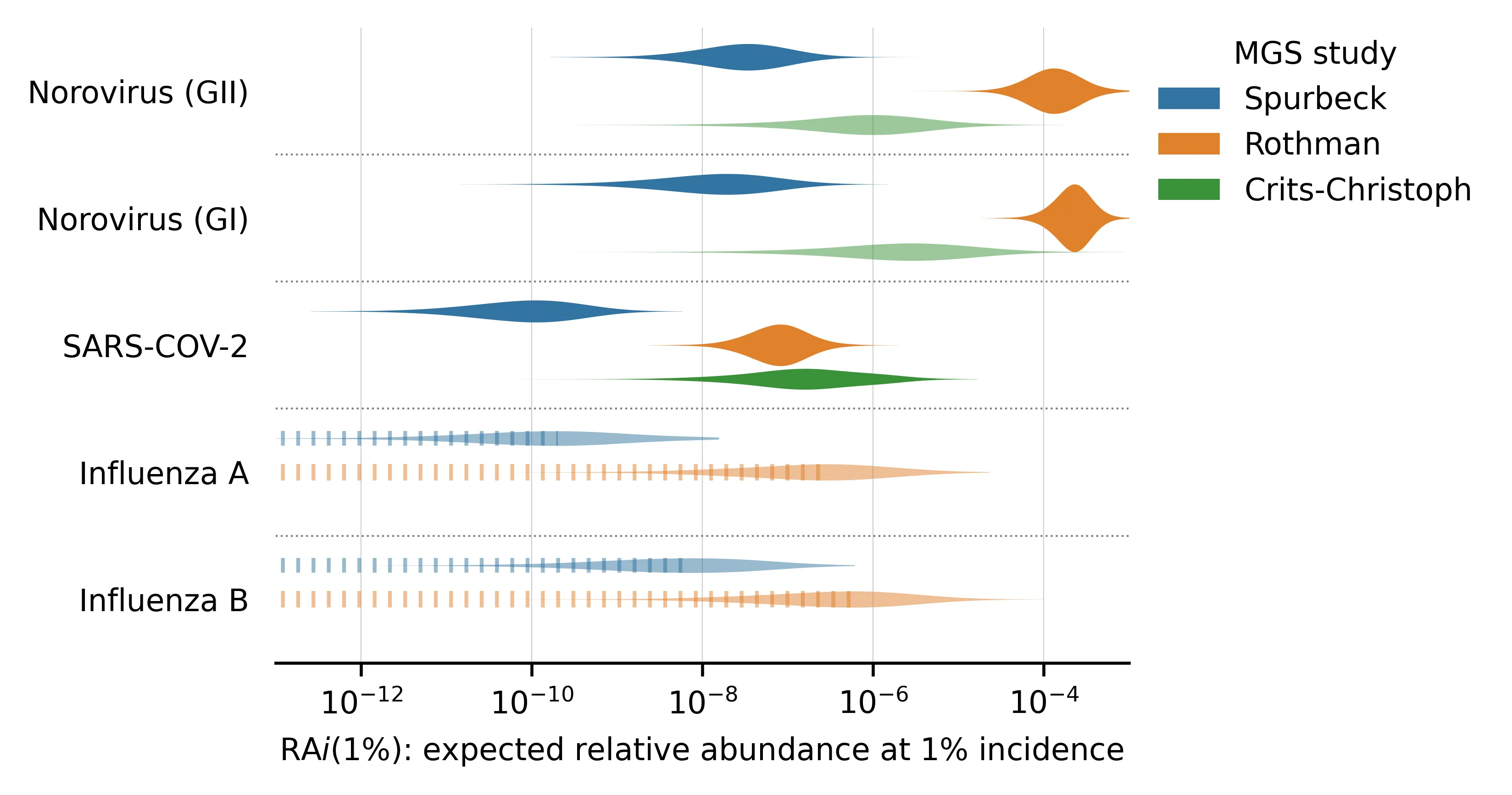
We've sorted the viruses by the total number of samples with any reads matching the virus.
Here is a similar plot, showing the posterior distributions of for viruses with prevalence estimates. These are all chronic viruses, and all but the first two (HIV and HCV) are DNA-based:
Figure 4: for viruses where we estimated prevalence.
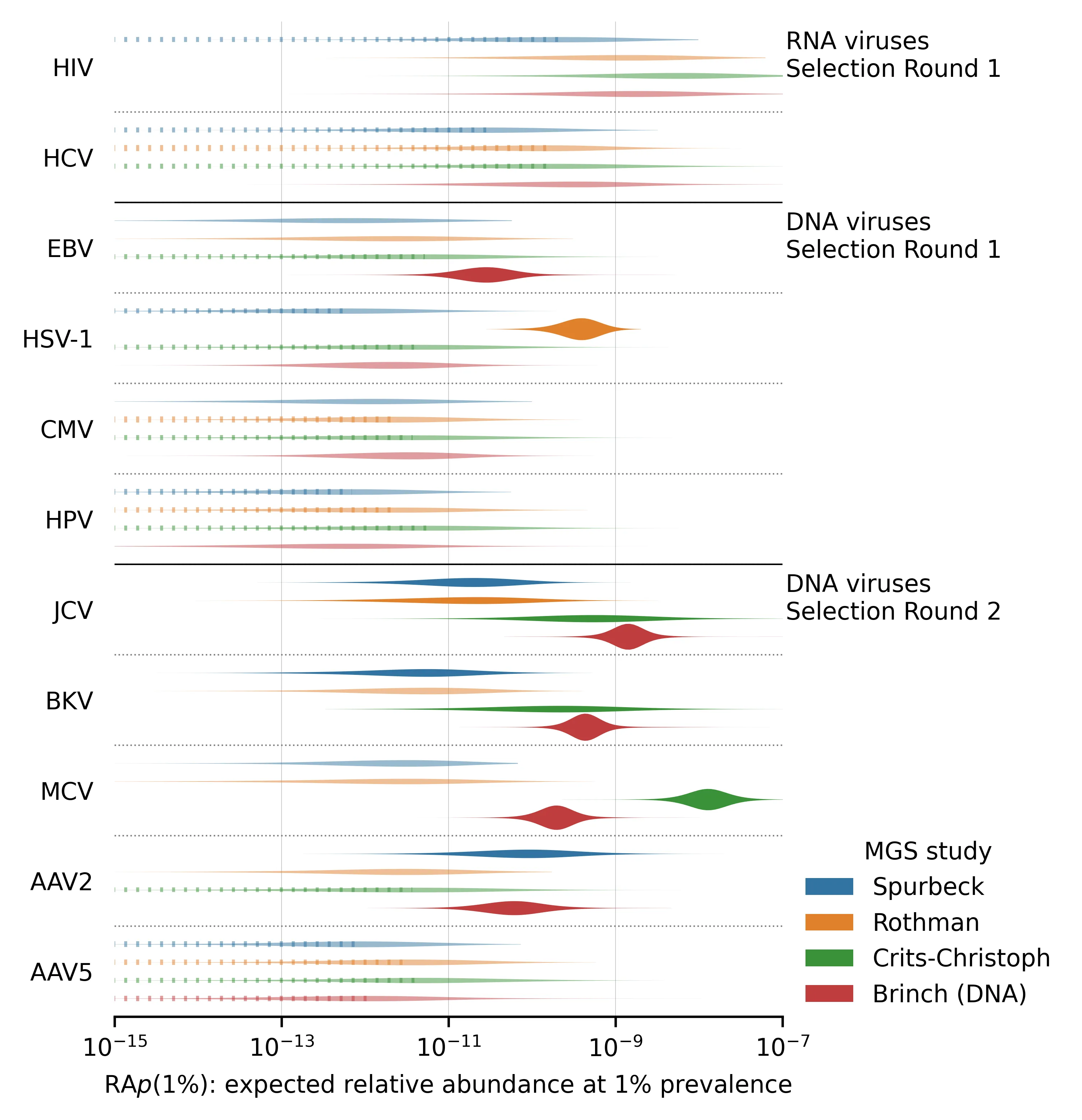
There are several notable aspects of these posterior distributions:
Even a pair of viruses that are both well-represented in the MGS data can have s that differ by several orders of magnitude. For example, compare norovirus (both genogroups) with median vs SARS-CoV-2 with median in the Rothman data. This makes sense, given that norovirus is primarily transmitted via feces whereas SARS-CoV-2 is primarily respiratory.
Different studies give very different estimates for a given virus and these differences are not consistent across viruses. For example, the estimated is higher in Rothman than Crits-Christoph for both norovirus genogroups but lower for several others (e.g., JCV, BKV, and MCV). This suggests that the differences in sample processing are meaningful for determining relative abundance.
For viruses with no observed reads (e.g., influenza A and B), our estimate of still varies between studies. This is because the total read counts and public health predictors can vary between studies. Observing zero reads sets an upper bound on the plausible . When total read count or incidence/prevalence is higher, this bound is lower and vice versa.
The DNA study, Brinch, has many more reads than the three RNA studies and thus tends to have sharper parameter estimates. You might expect that as a DNA study it would have consistently higher for DNA viruses than the RNA studies, but this isn't what we found in every case. For example MCV has a higher in Crits-Christoph (RNA) than Brinch (DNA)
The Round 2 DNA viruses selected for having high read counts (JCV, BKV, MCV, AAV2) tend to have higher than the Round 1 DNA viruses, reflecting the aforementioned selection bias.
Expected Relative Abundance by Sampling Location
We can also use our hierarchical model to estimate expected relative abundance separately for each sampling location. Below are plots of estimates for the three most abundant acute-infection viruses, separated by sampling location.
Figure 5: for the three most abundant acute viruses.
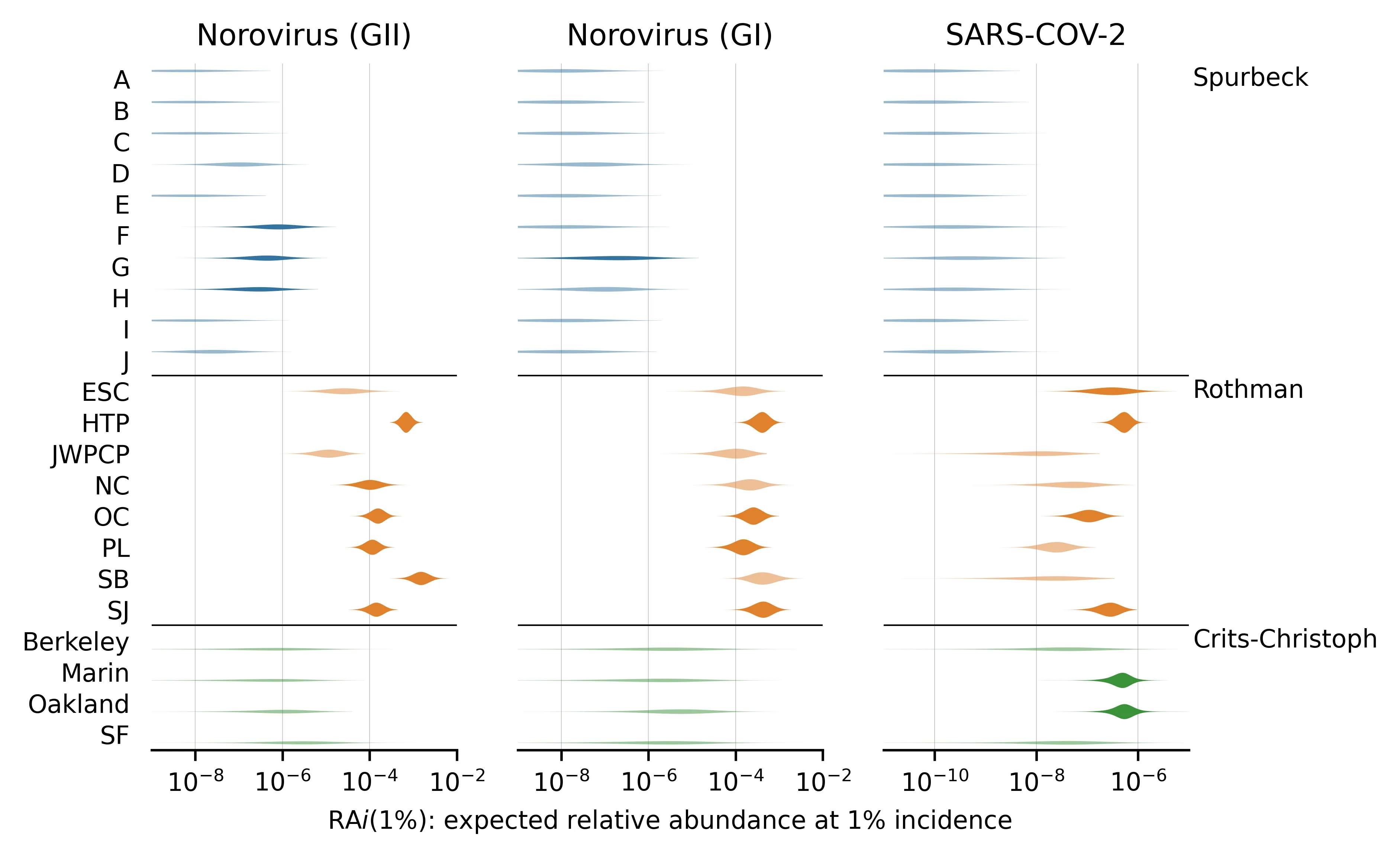
One reason locations within a study might be expected to vary in is that some studies used different sample preparation methods at different locations. For example, in Spurbeck, only locations E, F, G, and H used concentrating pipette ultrafiltration,[10] which selects for viral particles. Consequently, locations E through H tend to have higher estimates than the other Spurbeck locations, though estimates are still lower than in the Crits-Christoph or Rothman studies.
We also see signs of between-location variation in in the Rothman study. For instance, posterior median for SARS-CoV-2 is 10 times higher for HTP than for NC, and is even higher compared to JWPCP, which has no SARS-CoV-2 reads. These comparisons are roughly consistent across the three viruses, suggesting that there may be differences in how these samples were handled or collected.
There is also some evidence of virus/location interaction effects. The SB site in Rothman has higher than average for norovirus, but no SARS-CoV-2 reads at all.
For corresponding plots of , estimates for the three most abundant chronic-infection viruses, see Appendix C.
Example Application of
One key question the NAO is interested in is how effective pathogen-agnostic metagenomic sequencing of wastewater could be at detecting a novel pandemic. To illustrate how our results could be used in answering this question, here's a rough overall model:
Imagine your goal is to catch a pandemic when some fraction of people have been infected. As a first approximation, catching something when half as many people have been infected would cost about twice as much because it requires about twice the sensitivity.
For simplicity, let's say we want to detect a pathogen when 1% have been infected. The weekly incidence corresponding to a cumulative incidence of 1% will depend on the growth rate—with a shorter doubling period you'll have a higher weekly incidence when reaching that 1% threshold than with a longer one—but imagine it's spreading with a doubling period of a week (10% daily growth). Then when 1% of people have been infected approximately half of them will have been infected within the last week, giving a weekly incidence of 0.5%.
If the virus and sequencing approach were similar to SARS-CoV-2 in Rothman 2021, where we found a median of 8e-8, would be 4e-8 (1 in 3e7 reads). Then, if you need one thousand reads matching the virus in the most recent week to flag it for manual followup[12] you would need a sequencing depth of approximately 3e10 weekly reads to flag the sequence. If you're paying $8k per billion reads,[12] this would cost $200k/week or $11M/year (calculations).
Alternatively, imagine the virus and you're modeling is more similar to EBV in Brinch, where we used prevalence as the public health predictor and found a median of 3e-11 (1 in 4e10 reads). If you still need 1,000 reads matching the virus this implies a sequencing depth of 4e13 and an impractically high cost of $300M/week ($15B/year).
On the other hand, if instead of trying to identify a novel virus you have a list of concerning genomes and want to know if any appear, the required sequencing is much lower. Consider the same two scenarios, but instead of needing 1,000 matching reads you only need, say, three. Then costs would be more like $30k/year for SARS-CoV-2 in Rothman and $45M/year for EBV in Brinch.
Given the limitations noted below, however, these rough cost estimates should be taken with a large grain of salt.
Discussion
We connected pathogen incidence and prevalence data to pathogen relative abundances in wastewater, producing estimates of . This gives us an initial idea of the expected relative abundance for different methods and viruses, and allows us and others to narrow down the likely costs of metagenomic sequencing of wastewater for viral surveillance. While this report does not provide a comprehensive survey of either human viruses or sample collection and processing, it presents a general approach that can be applied to new viruses and metagenomic sequencing datasets to gradually expand our understanding of .
Impact of Sequencing Methods
One of the largest differences between studies, and in some cases between sites in a single study, is their approach to sequencing preparation. For example, in Spurbeck sites E, F, G, and H used a single method ("Method 4" in their paper) and most viruses have a higher at those sites. Could this also explain the large differences between human viral fractions we saw between studies in Table 1, and indicate that optimizing sequencing methods should be a high priority? For example, our reanalysis of Yang et al. (2020) gave a relative abundance of human viruses of 2e-4, which is 50-100x higher than what we saw in our the four studies we focused on. When we looked at which viruses this represented, however, we found that this high relative abundance was driven almost entirely by fecal-oral viruses like Salivirus and Astrovirus. Yang et al. were sampling in Urumqi, Kashgar, and Hotan in China's Xinjiang province while our four main studies were in the United States and Denmark: it's quite plausible that, due to differences in sanitation, this reflects differences in prevalence instead of sequencing method. There may or may not be a large potential for gains from optimization; this isn't something our data sheds much light on.
Limitations
While we think this work is a useful step toward predicting relative sequence abundance as a function of viral prevalence, it has a number of important limitations.
Metagenomic sequencing data
The total amount of sequencing data we were able to use was 7B reads (~$60k in sequencing at bulk prices[11]). While this is a lot of reads compared to many individual studies, we still had zero reads for some of our target viruses, especially rare viruses and chronic infections, and can only give weak upper bounds on their . While these upper bounds are useful in informing the lower bounds of detection cost estimates, more data would help a lot here.
We hoped to draw conclusions on which methods might be most suitable for the kind of monitoring we envision, but the studies were not generally set up to collect the kind of data that would support those comparisons. Studies were at different times and places, and weren't trying to facilitate this kind of comparison.
We were unable to find a suitable metagenomics study that used a virally-enriched DNA sequencing protocol.
Public health data
The public health estimates generally include a factor for underreporting, and these factors are one of the weakest parts of the estimates. For instance, in SARS-CoV-2 they act as a uniform factor, applied across two years of testing data and different SARS-CoV-2 variants.
Three out of four studies we selected used RNA sequencing but we weren’t able to create as many RNA virus public health estimates as expected. Many obvious seasonal RNA target viruses had poor publicly available incidence data (metapneumovirus, rhinovirus) or were at close to zero incidence during the metagenomic sampling periods (respiratory syncytial virus), making time-resolved estimates of these viruses impractical or low-value. For future work, sampling during a time period that typically sees surges in RNA virus prevalence, such as RSV or influenza season, would be valuable.
The public health predictors we were able to collect were often provided as point estimates of incidence or prevalence. In cases where there was information about the potential range they weren't provided in a consistent manner, and while we did collect them, we did not incorporate that information into the model.
Our round two viruses with the exception of AAV5 (AAV2 and the polyomaviruses) were chosen because they appeared in sequencing data. That we observed hundreds of reads for AAV2 and none for the nearly-as-prevalent AAV5 suggests that this step introduced strong selection effects.
We can’t distinguish whether differences between two studies are due to real differences in or systematic, unobserved biases in the public health predictors. For example, if public health agencies in a particular state have abnormally high rates of case undercounting, the inferred will be artificially higher in MGS studies performed there.
Modeling
Our model assumes that the errors in our estimates of the public health predictors are independent between samples. In fact, we would expect them to be autocorrelated in both time and space. For example, consider a virus for which we have only annual incidence estimates from the United States as a whole. If there were an outbreak in Orange County in May, 2021, our estimate will be wrong in the same direction for all the samples in that region at that time.
Our model also only represents sample preparation methods indirectly through the sample-location terms, and so does not provide an explicit estimate of its effect. However, such an estimate would be difficult to obtain reliably from this small collection of studies.
- Similarly, we do not directly infer any effects of viral properties (DNA vs RNA, enveloped vs not, etc). In principle, we could create a larger model that estimates for all viruses simultaneously and includes some of these properties as factors. Because we only have public health estimates for about a dozen viruses and those are split between incidence and prevalence, however, we decided that fitting such a model would not be worthwhile with this data set.
Future work
To more systematically estimate the cost of detecting a wide range of potential viral pandemics, we are developing a model of the entire detection process of an operational NAO, including the spread of the virus in the population, the design of the monitoring system (sampling frequency and depth), sample preparation and sequencing (the model described in this report), and statistical methods for flagging sequences of concern. The structure and parameterization of this model will be directly informed by the present study.
We hope to expand this analysis to cover more viruses and metagenomics datasets. Acute-infection viruses like influenza, respiratory syncytial virus, and seasonal coronaviruses were heavily suppressed by the COVID-19 pandemic, so we're enthusiastic about analyzing data from the winter 2022-2023 and 2023-2024 seasons. Highly-prevalent DNA viruses tended to have very low and uncertain in the non-virally-enriched DNA dataset we analyzed (Spurbeck); including a virally-enriched DNA sequencing dataset may give sharper estimates for as well as the quantitative benefit of viral enrichment for DNA sequencing protocols.
Appendix A: Public Health Data
Below we summarize the methods we used to estimate the public health predictors for each virus. We've put incidence viruses first, and then sorted the table by how much of our own adjustment we needed to apply on top of our input estimates. In general, our results will be most robust in cases where we only required minimal adjustment to trustworthy external estimates (ex: HSV-1 in the US where the CDC generates a prevalence estimate), and least when we needed more (ex: EBV in Denmark where we extrapolated 1983 Danish seroprevalence results to modern Denmark's age structure).
Table 5: methods used to estimate each public health predictor.
| Virus | Selection | Predictor | Underlying Data for US | Underlying Data for Denmark |
|---|---|---|---|---|
| SARS-CoV-2 | Round 1 | Incidence | Confirmed and probable COVID-19 cases (source), adjusted by a CDC-estimated underreporting factor | No estimate |
| Influenza A&B Virus | Round 1 | Incidence | Number of positive tests, adjusted by a yearly underreporting factor (official_yearly_incidence/yearly_positive_tests) | No estimate |
| Norovirus | Round 1 | Incidence | Using a yearly incidence estimate from 2006, we then adjust this incidence for a given time period, by dividing the average number of norovirus outbreaks, per time period, by the actual number of norovirus outbreaks, for that time period. | No estimate |
| Herpes Simplex Virus 1 (HSV-1) | Round 1 | Prevalence | CDC estimates of HSV-1 seroprevalence among 14-49 yos. Based on measurements of 3710 individuals as part of the NHANES cycle 2015-2016. Rates are likely similar today, as there is still no vaccine. | Weighted seroprevalence data based on a 2008-2011 survey of 6627 Germans.). Extrapolated to Denmark. |
| Herpes Simplex Virus 2 (HSV-2) | Round 1 | Prevalence | CDC estimates of HSV-2 seroprevalence among 14-49 yos. Based on measurements of 3710 individuals as part of the NHANES cycle 2015-2016. Rates are likely similar today, as there is still no vaccine. Dropped for bioinformatic limitations. | Weighted seroprevalence data based on a 2008-2011 survey of 6627 Germans.). Extrapolated to Denmark. |
| Cytomegalovirus (CMV) | Round 1 | Prevalence | Raw data of CMV seroprevalence. Data was obtained in the NHANES cycle 1999-2004, among 15,310 participants. CMV has no vaccine, so rates should stay approximately constant. | 2006 seroprevalence measurement of 19,781 sera from the Netherlands. Extrapolated to Denmark. |
| Epstein-Barr-Virus (EBV) | Round 1 | Prevalence | CDC EBV seroprevalence measurements, adjusted for demographics. Data was obtained in the NHANES cycles 2003-2010, among 6 to 19 year olds. Based on EBV’s lifelong latency, measurements among 18-19 year olds were taken as representative of the adult population. | 1983 EBV seroprevalence measurements in 518 Danish children and 178 adults. Applied to Denmark by adjusting for Denmark’s age structure. |
| Human Immunodeficiency Virus (HIV) | Round 1 | Prevalence | Using a CDC estimate of all infected individuals, we scale this estimate by the share of HIV-positive individuals who are non-HIV-suppressed. | Estimated undiagnosed HIV-positive individuals, provided by the Danish Statens Serum Institut. Scaled by share of HIV diagnoses occurring in Copenhagen. |
| Hepatitis B Virus (HBV) | Round 1 | Prevalence | Chronic Hep B case estimates by a panel of US hepatologists. Denmark estimates are based on a domestic prevalence estimate. Dropped for bioinformatic limitations. | Estimate of total HBV cases in Denmark, provided by Danish researchers. |
| Hepatitis C Virus (HCV) | Round 1 | Prevalence | Chronic Hep C case estimates by CDC researchers. | Estimate of total HCV cases in Denmark, provided by Danish researchers |
| Human Papilloma Virus (HPV) | Round 1 | Prevalence | CDC HPV prevalence measurements, adjusted for demographic biases. Data was obtained in the NHANES cycle 2013-2014 and 2015-2016. | HPV PCR measurements in a 2016 male Danish cohort of 2436 men |
| Adeno-Associated Viruses (AAV-2, AAV-5, AAV-6) | Round 2 | Prevalence | Extrapolating seroprevalence measurements in hemophilia patients (demographic composition), both for the US and Denmark. Dropped AAV6 for bioinformatic limitations. | 2022 seroprevalence measurements among hemophilic patients from several countries. We aggregated measurements from France, Germany, and the UK, extrapolating the result to Denmark. |
| John-Cunningham Virus (JCV) | Round 2 | Prevalence | US estimates are based on a US seroprevalence survey of healthy adult blood donors. | Swiss seroprevalence study of 400 healthy adult blood donors. Extrapolated to Denmark. |
| BK Virus (BKV) | Round 2 | Prevalence | US estimates are based on a US seroprevalence study of healthy adult blood donors. | Swiss seroprevalence study of 400 healthy adult blood donors. Extrapolated to Denmark. |
| Merkel Cell Virus (MCV) | Round 2 | Prevalence | US estimates are based on a US seroprevalence study of 451 female control subjects. | Dutch seroprevalence study) of 1050 serum samples. Extrapolated to Denmark. |
Appendix B: Bioinformatic Details
We downloaded the data from the SRA to Amazon S3 as raw paired-end reads in compressed FASTQ format. We then processed the data with a custom pipeline (GitHub) to determine how many reads belonged to each target virus. First we ran AdapterRemoval2 v2.3.1 to remove adapters, trim low-quality bases, and merge overlapping forward and reverse reads. Then we ran Kraken2 to assign each read to a clade (a node in the taxonomic tree). We used the 2022-12-09 build of the Standard 16GB database, which includes reference sequences for viruses, along with archaea, bacteria, plasmids, and humans. This database is capped at 16GB to reduce memory requirements, which slightly reduces sensitivity and accuracy relative to the uncapped (67GB) database.
We validated that our Kraken configuration was able to assign reads appropriately by checking what fraction of 100-mers from the canonical RefSeq entries for each target virus Kraken was able to assign to that virus (code). Sensitivity ranged from 98% (AAV5) to 84% (HSV-1). At this stage we realized that HBV, HSV-2, and AAV6 were not in the Standard 16GB database: HBV and HSV-2 only have scaffold-quality RefSeq genomes and AAV6 is not in RefSeq at all. We dropped all three from our analysis.
We identified duplicate reads within a sample by exact match on the first and last 25 bases, and counted groups of duplicate reads only once in our analysis.
To assess and remove false positives, we took the reads Kraken2 identified, aligned them to the reference genomes, and computed a percent-identical score for each read. For each virus we manually evaluated a selection of reads with different scores. This involved viewing the alignment and querying BLAST, and in many cases what looked like a poorly matching read when evaluated against the RefSeq genome was a much better match for a variant BLAST was able to find in GenBank. Many viruses, however, had a score below which all manually-inspected reads were a better fit for something else in GenBank, and we did not count those reads in our analysis (code). We discarded 17 reads for CMV, 16 for HSV-1, and one each for AAV5, EBV, HCV, and influenza A.
Appendix C: Statistical Analysis Details
Predicting Expected Relative Abundance
Above we assumed:
Using natural logarithms and letting , we can rewrite the previous equation as
or more compactly
Our goal is to estimate the parameter . In the language of regression models, is the intercept term of a logistic regression of the relative abundance on the logarithm of the public health predictor, with the slope term fixed at 1.
Once we have an estimate of , it is useful to transform the result into something more biologically interpretable. Above we defined the quantity to be the expected relative abundance when the public health predictor is equal to one person per hundred. We can compute as:
Statistical Model
We estimate and for each virus in each metagenomic study separately with the following Bayesian model. In each study, we have metagenomic samples taken at various times from sampling locations. For sample , our data consist of the total number of reads , the number of viral reads , and the public health predictor (prevalence or weekly incidence depending on the virus). We fit a hierarchical logistic regression model to estimate the intercept term , as defined above. Because some MGS studies use different sample preparation methods for different sampling locations and because our preliminary analysis suggested per-location variation in the for SARS-CoV-2 in the Rothman dataset, we use a hierarchical model with a separate intercept term for each sampling location. The hierarchical model allows us to jointly estimate the location-specific effects and an overall coefficient for the study and virus.
We define a parameter to represent the “true” log relative abundance of focal viral nucleic acid contributing to the sample. It accounts for three factors:
error in our estimate of the public health predictor
differences between the population the estimate is derived from (e.g., the entire United States for all of 2021) and the population contributing to the sample (e.g., Orange County on May 21, 2021)
unbiased noise in the read counts that’s not accounted for by the binomial model.
We model the viral counts in each sample as a binomial random variable:
The proportion parameter of the binomial follows the form justified above.
We assign a prior distribution, centered on the public health estimate, as:
Because we don’t a priori know , the standard deviation of , we learn it from the data, using the prior . This distribution avoids zero and has a mode at one, representing the belief that our estimated public health predictors will vary from the truth somewhat, but not by many orders of magnitude.
Finally, we have an intercept term where is the location of the sample. Our hierarchical model of intercept terms has the structure:
Here, is the overall intercept for the study and virus and is the standard deviation of the location-specific terms around this overall value. The prior on is centered on , where a bar represents an average across samples. We chose this parameterization so that roughly represents the naive estimate you would get by dividing the relative abundance in all of the data by the average prevalence estimate across samples. This sort of centering is common in applied Bayesian inference because it improves the numerical stability of the estimation algorithms. We aimed to have the prior on be weakly informative: it supposes that the naive approximation is not off by more than a few orders of magnitude, but does not contain any other substantive scientific information. Thus we chose a prior standard deviation on b to be as large as possible while still allowing for efficient sampling (see Model Checking).
As with , we learn from the data, allowing for some studies to have a lot of variation between sampling locations and others to have little.
We fit the model with Stan, as described above, generated samples of and , and transformed them to find the more biologically interpretable .
Model Checking
To assess the posterior sampling, we examined plots of the marginal and joint posterior distributions of the parameters. Posterior distributions that have irregular “spikes” at particular values or are strongly multimodal indicate that the HMC sampler may not be exploring the parameter space efficiently, likely due to model specification issues. We also compared the prior and posterior distributions to ensure that the priors did not have undue influence on the posteriors. For example, we found that our initial choice of prior was too narrow, significantly constraining the posterior distribution even for the virus/study combinations with a lot of data. Conversely, we found that was too broad, leading the sampler to mix poorly. Similarly, we adjusted the priors on and to avoid the lower bound at zero.
To check the fit of the model, we used the posterior samples of the model to generate simulated datasets. We compared the simulated data to the observed data, looking for features of the data not accurately captured by the model. For example, an earlier version of the model did not include terms for sampling locations within studies. Posterior predictive checks revealed that this model failed to predict the low read counts for SARS-CoV-2 in the Point Loma (PL) location of the Rothman dataset, inspiring us to add location-specific effects.
by Sampling Location for Chronic Viruses
Figure 6: for the three most abundant chronic viruses.
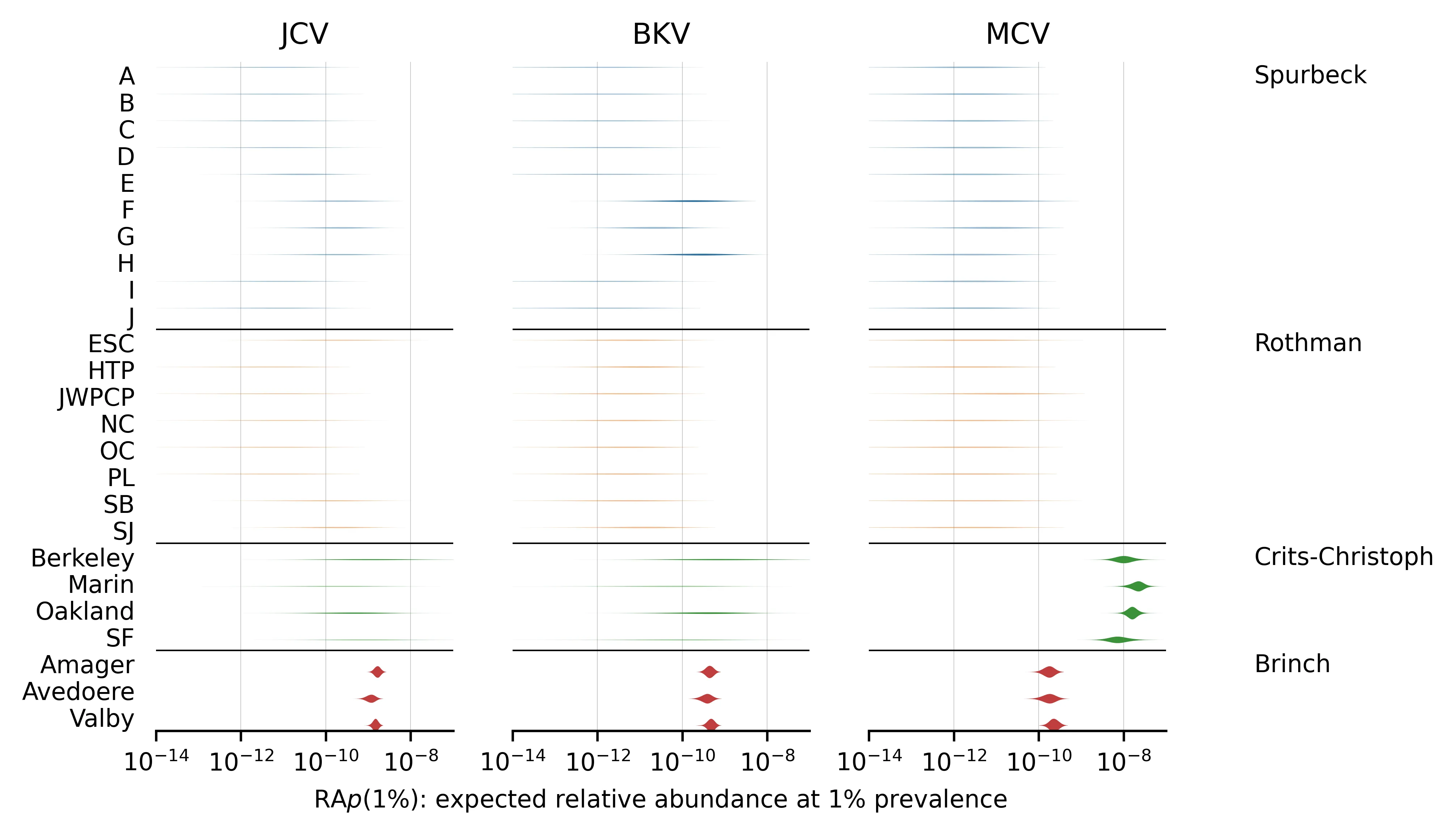
Note that the estimates for Spurbeck and Rothman are based on very few reads.
Footnotes
- ↩
Adrian Hinkle, Alexander Crits-Christoph, Alexandra Alexiev, Amity Zimmer-Faust, Ana Duarte, Angela Minard-Smith, Anna Charlotte Schultz, Anne Mette Seyfarth, Antarpreet Jutla, Anthony Smith, Anwar Huq, Asako Tan, Avi Flamholz, Barry Fields, Basem Al-Shayeb, Berndt Björlenius, Bing-Feng Liu, Boonfei Tan, Bradley William Schmitz, Bram van Bunnik, Brian Fanelli, Camille McCall, Carl-Fredrik Flach, Chandan Pal, Changzhi Wang, Charmaine Ng, Ching-Tzone Tien, Chiran Withanachchi, Chiranjit Mukherjee, Christian Brinch, Christian Carøe, Christina Svendsen, Corinne Walsh, Cresten Mansfeldt, D Joakim Larsson, David Mantilla-Calderon, David Wanless, Defeng Xing, Dilini Jinasena, Dongmei Yan, Elías Stallard-Olivera, Emily Kibby, Eric Adams, Eric Ng’eno, Eric Peterson, Erik Kristiansson, Fanny Berglund, Francis Rathinam Charles, Frank Aarestrup, Fred Hyde, Frederik Duus Møller, Gary Schroth, Godfrey Bigogo, Guo-Jun Xie, Haishu Tang, Hamed Al Qarni, Han Cui, Hannah Greenwald, Hannah Holland-Moritz, Harpreet Batther, Henrik Hasman, Hongjie Chen, Isaac Zhou, Jacob Bælum, Jacob Jensen, Jane Carlton, Jason Rothman, Jeffery Koble, Jeffrey Chokry, Jennifer Verani, Jerker Fick, Jessica Henley, Jette Kjeldgaard, Jillian Banfield, Jing Wang, Joel Montgomery, Johan Bengtsson-Palme, John Griffith, John Neatherlin, John Sterrett, Jonathan Hetzel, Joseph Cotruvo, Joseph Kapcia, Joshua Steele, Julia Maritz, Kara Nelson, Karina Gin, Karlis Graubics, Katherine Dyson, Katherine Ensor, Katrine Whiteson, Kristine Wylie, Kun Feng, Kyle Brumfield, Kyle Schutz, Kylie Langlois, Lasse Bergmark, Lauren Kennedy, Lauren Stadler, Laurence Haller, Liam Friar, Lindsay Catlin, Loren Hopkins, Lucy Mao, Madison Griffith, Malinda Wimalarante, Manoj Dadlani, Marcus Östman, Marion Koopmans, Mark Woolhouse, Mathis Hjelmsø, Mats Tysklind, Matthew Gebert, Matthew Olm, Menu Leddy, Mohsen Alkahtani, Moiz Usmani, Na Xie, Nathaniel Registe, Nicholas Dragone, Noah Fierer, Oksana Lukjancenko, Ole Lund, Onyango Clayton, Oscar Whitney, Patrick Munk, Pei-Ying Hong, Pierre Rivailler, Pimlapas Leekitcharoenphon, Qian Yang, Rachel Spurbeck, Rene Hendriksen, Rickard Hammarén, Rita Colwell, Rose Kantor, Rushan Abayagunawardena, Ryan Doughty, Ryan Leo Elworth, S Elizabeth Alter, Samuel Kiplangat, Sara Spitzer, Sarah Gering, Scott Kuersten, Shuangli Zhu, Sierra Jech, Simon Rasmussen, Susanne Karlsmose, Suzanne Dorsey, Sünje Pamp, Theresa Loveless, Theresa Ten Eyck, Thomas Petersen, Thomas Sicheritz-Pontén, Timo Röder, Tina Melie, Tine Hald, Todd Treangen, Todd Wylie, Tong Zhang, Traoré Oumar, Wenbo Xu, William Patterson, Xiao-Tao Jiang, Xiaoqiong Gu, Xiaoyu Cai, Yanghui Xiong, Yasir Bashawri, Yong Zhang, Yue Clare Lou, and the Global Sewage Surveillance Consortium.
- ↩
Spurbeck doesn’t provide information on the methodology of sample acquisition, but the Ohio Coronavirus Wastewater Monitoring Network (OCWMN), from which the authors received extracted RNA, notes online that they take 24-hour composite samples at the WTP inlet.
- ↩
Brinch: Illumina MiSeq, 2×250, and NextSeq 550, 2×150. Crits-Cristoph: Illumina NextSeq 550, 2×75bp, Rothman: Illumina NovaSeq 6000 2×100bp or 2×150bp, Spurbeck: Illumina NextSeq 500/550, 2×150bp.
- ↩
Having prevalence for some viruses and incidence for others is not ideal: we'd much rather get everything into consistent terms to allow better comparisons between viruses and to simplify the discussion and interpretation of our results. Initially we planned to standardize on some kind of prevalence, but ran into several issues:
For an acute infection there are many ways you could operationalize "prevalence": do we want the number of people who have symptoms, are currently infectious, are shedding into wastewater, or something else? And how do you handle that these categories are not binary? For instance, viral shedding will vary over many orders of magnitude in each person as an infection progresses.
The quantity that we actually expect to be proportional to wastewater counts is something like shedding-weighted prevalence, where someone who is maximally infectious and shedding many copies counts more than someone with a lingering infection shedding just a few. But estimates of this quantity are not readily available.
If the vast majority of shedding from a typical acute infection is within just a few days, then—since the time resolution of our public health data was approximately weekly—the potential accuracy improvement from modeling shedding dynamics more finely would be minimal.
In applying our results, however, we expect people to be working with epidemiological models that generate both incidence and prevalence at each timestep. This means they can use our incidence estimates for viruses where we provide them, and prevalence estimates for the remaining ones.
- ↩
Only rarely did we find credible sub-national prevalence estimates for chronic infecting viruses.
- ↩
The CDC estimated the COVID-19 underreporting factor for February 2020 - September 2021, which doesn’t take into account the November 2021 emergence of the Omicron variant. Given the large number of asymptomatic Omicron infections, it is thus likely that using a uniform, pre-Omicron underreporting factor underestimates true Omicron incidence.
- ↩
SARS-CoV-2 and influenza incidence rates are averaged across the covered regions, adjusting for population. E.g., influenza incidence is a weighted average of Ohio and California incidence, weighted by the relation of Ohio’s and California’s population.
- ↩
COVID-19 suppression also reduced Respiratory Syncytial Virus (RSV) infection rates, with the CDC noting that the expected 2020/2021 RSV season “did not occur”. After the winter of 2020/2021, RSV remained so uncommon in our target areas and times that we decided not to create estimates.
- ↩
We predicted this effect would only be significant for Crits-Christoph: influenza counts were zero for 100% of samples, so our estimate of should be driven entirely by the choice of pseudocount. For Rothman, we expected the estimate to be driven by the majority of samples with non-zero incidence. For Spurbeck, very few samples had zero incidence and many samples had very high incidence, so we expected a minimal effect. To test our expectations, we performed a sensitivity analysis by substituting a pseudocount that was 100x smaller (0.001 instead of 0.1). In the case of Crits-Christoph we did indeed find was driven entirely by the choice of pseudocount. For Rothman, however, we found the 95th percentile estimate for influenza's increased by only 22%, and in Spurbeck it was unchanged.
- ↩
The Spurbeck study does not provide a lot of detail on the different methods used, plausibly because the WTP operators, not the authors, ran the protocols.
- ↩
Imagine you're using a k-mer based detection system where you need to see the same k-mer from week to week. Then only (ReadLength - k) / GenomeLength of your reads will match that k-mer. Say the virus is 16,000 bp, you're doing 2x150 sequencing that gives you 200 bp average reads after trimming, and you set k=40: that's (200-40)/16,000 or 1% of your reads that hit the virus hitting any given one of its 40-mers. Then figure that due to noise and avoiding false positives you need to see your target k-mer ten times in your most recent week to flag it as suspicious, and we get a factor of 1,000.
- ↩
The MIT BioMicroCenter charges $14,850 per flow cell for NovaSeq S2 300nt sequencing. Double this to include library prep and other costs. A NovaSeq 6000 with an S2 flow cell is advertised as giving 1-1.25TB of data at 2x150, or 3.3B-4.1B read pairs. Then the cost is ~$8k per billion read pairs. This will likely go down: Illumina has recently released the more cost effective NovaSeq X, and as Illumina's patents expire there are various cheaper competitors.